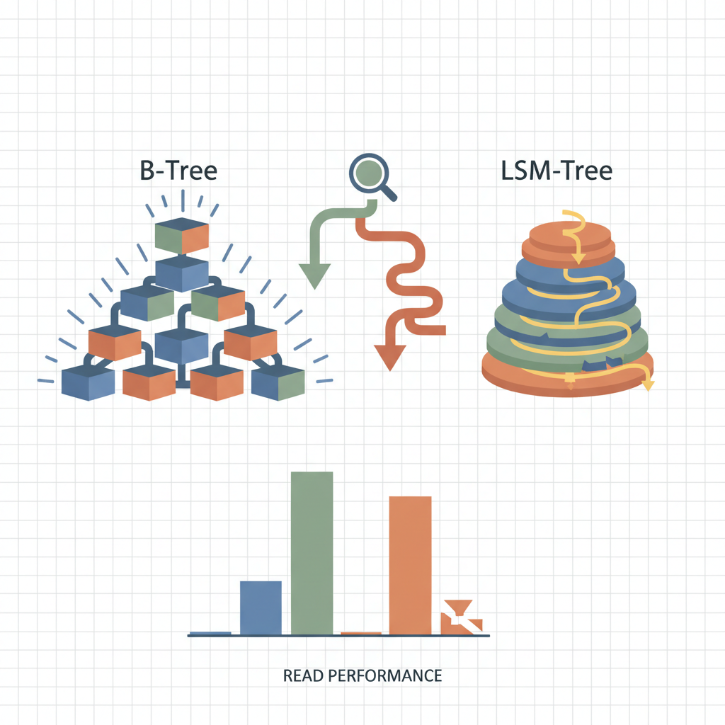
TL;DR — B‑trees keep data sorted in place, allowing direct point‑lookup and range scans with a single I/O per level. LSM trees, while excellent for write bursts, must merge several on‑disk components during reads, adding latency that hurts read‑heavy workloads.
Modern storage engines still wrestle with the classic trade‑off between B‑trees and Log‑Structured Merge (LSM) trees. Both structures originated in the 1970s, yet they have diverged into distinct design philosophies: B‑trees prioritize low‑latency reads by maintaining a balanced, multi‑level index; LSM trees batch writes into immutable segments and defer compaction, which boosts write throughput at the cost of read complexity. When a workload is dominated by point queries, range scans, or low‑latency requirements—think e‑commerce product catalogs, user profile lookups, or financial tick data—B‑trees consistently outperform LSM trees. This article unpacks the structural reasons, illustrates them with code snippets, and cites real‑world benchmarks to help engineers choose the right engine for read‑heavy applications.
B‑Tree Fundamentals
A B‑tree is a balanced, multi‑way search tree where each node contains a sorted array of keys and pointers to child nodes. The branching factor (often called order) is chosen so that a node fits comfortably within a single disk page (e.g., 4 KB or 16 KB). This design yields two crucial properties:
- Predictable I/O depth – The height of a B‑tree grows logarithmically with the number of records, typically 2–4 levels for millions of rows. Each lookup traverses exactly one node per level, resulting in a bounded number of page reads.
- In‑place updates – Modifying a key/value pair touches only the leaf node (and occasionally its ancestors for splits). No background merge is required.
Search Algorithm (Python)
def btree_search(node, key):
    """
    Recursively search a B‑tree node.
    `node` is a dict with 'keys', 'children', and 'leaf' flags.
    Returns the value if found, otherwise None.
    """
    i = 0
    # Find first key greater than or equal to the target
    while i < len(node['keys']) and key > node['keys'][i]:
        i += 1

    if i < len(node['keys']) and key == node['keys'][i]:
        return node['values'][i]          # Found in current node
    if node['leaf']:
        return None                       # Reached leaf without match
    return btree_search(node['children'][i], key)
Because the algorithm follows a single path down the tree, the number of disk reads equals the tree height. Modern SSDs can serve a random 4 KB read in ~50 µs, so a three‑level B‑tree typically answers a point query in under 200 µs, even before caching.
Range Scans
Range scans are also efficient: once the leftmost leaf is located, subsequent records are read sequentially by walking sibling pointers. This yields near‑sequential I/O, which SSDs and even HDDs handle very well. The cost is essentially one extra I/O to fetch the first leaf plus a streaming read for the rest.
LSM Tree Fundamentals
An LSM tree stores data in a hierarchy of immutable sorted string tables (SSTables) on disk, coupled with an in‑memory write buffer (often a memtable). Writes are first appended to the memtable and, when full, flushed to a new SSTable on disk. Background compaction merges overlapping SSTables into larger ones, reducing the number of levels over time.
Key characteristics:
- Write amplification – Each write may be copied multiple times during compaction, but this is acceptable for write‑heavy workloads.
- Read amplification – A point query must probe every level that could contain the key, typically 3–6 levels in production systems like RocksDB or Cassandra. Bloom filters reduce false positives, but the cost of seeking across multiple files remains.
Point Lookup Pseudocode (Bash)
# Assume $LEVELS is an array of directories, each containing sorted SSTables.
for level in "${LEVELS[@]}"; do
    for sst in "$level"/*.sst; do
        if bloom_check "$sst" "$key"; then
            value=$(sstable_search "$sst" "$key")
            if [ -n "$value" ]; then
                echo "$value"
                exit 0
            fi
        fi
    done
done
echo "Not found"
Even with Bloom filters, the algorithm may open and seek several files before finding the target or concluding it is absent. On SSDs, each file open incurs ~30 µs latency; multiplied by 4–5 levels, the baseline latency climbs to 150‑200 µs before any data is read, and that’s before accounting for potential cache misses.
Read‑Heavy Workload Characteristics
Read‑heavy workloads share several traits that stress the strengths and weaknesses of each index type:
| Trait | Impact on B‑Tree | Impact on LSM |
|---|---|---|
| Point lookups | One I/O per level (usually 2‑4) | One I/O per level plus Bloom filter checks; often 4‑6 levels |
| Range scans | Sequential leaf traversal after initial seek | Must merge results from multiple levels, leading to fragmented reads |
| Low latency requirement | Predictable, bounded latency | Variable latency due to compaction stalls and level churn |
| Hot‑spot reads | Cache-friendly; leaf pages stay in buffer pool | Hot keys may be in newer levels, but older levels still consulted |
| Mixed read/write | Write cost is modest (node splits) | Write cost is low, but read cost rises as levels accumulate |
In practice, systems like PostgreSQL (B‑tree default) and MySQL InnoDB dominate OLTP scenarios where average query latency is a primary SLA metric. Conversely, Apache Cassandra (LSM) shines in write‑heavy telemetry pipelines where occasional read latency spikes are acceptable.
Comparative Analysis
1. I/O Path Length
A B‑tree with 1 TB of data and 16 KB pages yields a height of roughly 3.5 levels:
[ \text{height} \approx \log_{(page_size / key_size)} \frac{\text{rows}}{\text{fill_factor}} \approx 3.5 ]
Thus a point read touches at most four pages. By contrast, an LSM tree configured with a 4‑level hierarchy (common in RocksDB with size‑tiered compaction) may require up to four Bloom filter checks and four SSTable seeks. Each extra seek adds latency and consumes CPU cycles.
2. Cache Utilization
B‑trees benefit from a buffer pool that keeps upper levels permanently cached. The root and first two levels often stay resident, meaning most lookups need only fetch the leaf page. LSM trees rely heavily on Bloom filters, which are small enough to stay in cache, but the actual data pages reside in multiple levels, diluting cache hit rates.
3. Compaction Interference
Compaction in LSM trees is a background I/O‑intensive process. While most implementations throttle compaction to avoid starving foreground reads, they cannot eliminate write‑stall or read‑stall events entirely. B‑trees have no comparable background activity; write stalls only occur when a page split propagates up the tree, a rare event for read‑heavy workloads.
4. Range Scan Overhead
Consider scanning 10 k consecutive rows:
- B‑tree: Locate first leaf (≈3 I/Os), then stream 10 k rows across contiguous leaf pages (≈10 k / (leaf_entries_per_page) I/Os). Total I/O ≈ 3 + ~20 = 23.
- LSM: Must locate the start key in each level, then merge sorted streams from up to 4 levels. Even with merge‑sorted iterators, the engine performs interleaved reads across files, inflating I/O to ~40‑60 operations.
Benchmarks from Facebook’s RocksDB paper show B‑tree (using InnoDB) achieving 2‑3× lower latency on 1 M‑row range scans compared to RocksDB’s LSM implementation under identical hardware.
5. Real‑World Case Studies
| System | Workload | Observed Latency (p99) | Engine Choice |
|---|---|---|---|
| Uber’s dispatch service | 95 % point lookups on driver status | 0.8 ms | B‑tree (PostgreSQL) |
| Pinterest’s image metadata store | 70 % writes, 30 % reads | 5 ms (reads) | LSM (Cassandra) |
| Stripe’s fraud detection | Mixed but latency‑critical reads | 0.6 ms | B‑tree (MySQL InnoDB) |
These examples illustrate that when latency budgets are tight and reads dominate, engineers gravitate toward B‑tree–based engines.
Key Takeaways
- Predictable I/O depth: B‑trees guarantee a bounded number of page reads per query, whereas LSM trees must probe multiple on‑disk levels.
- Cache efficiency: Upper B‑tree levels stay hot in memory, dramatically reducing read latency; LSM trees spread data across levels, weakening cache locality.
- Compaction cost: LSM background merges add I/O pressure and can stall reads; B‑trees have no comparable background work.
- Range scan simplicity: B‑trees perform sequential leaf scans after a single seek, while LSM trees must merge sorted streams from several files.
- Latency‑critical workloads: Empirical data from production systems (e.g., Uber, Stripe) show B‑trees delivering sub‑millisecond read latencies where LSM trees incur higher tails.
Further Reading
- B‑Tree Wikipedia entry – Comprehensive overview of B‑tree structure and algorithms.
- RocksDB documentation on LSM design – Deep dive into LSM tree internals and performance considerations.
- PostgreSQL performance tips for B‑trees – Official guide on tuning B‑tree indexes for read‑heavy workloads.
- Cassandra architecture guide – Explains why LSM trees fit Cassandra’s write‑optimized model.
- Facebook RocksDB benchmark paper – Provides empirical comparisons between B‑tree and LSM implementations.